partial least squares regression python

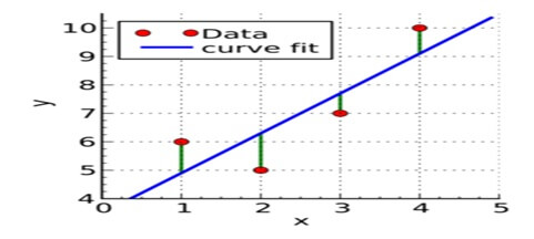
Partial least squares regression python : Green lines show the difference between actual values Y and estimate values Yₑ. The objective of the least squares method is to find values of α and β that minimize the sum of the difference between Y and Yₑ. We will not go through the derivation but using calculus we show the values of the unknown parameters are as follows:-

Least Square Regression
Where X̄ is the mean of X values and Ȳ is the mean of Y values.
If you are familiar with statistics, you may recognise β as simply
Cov(X, Y) / Var(X).
Ordinary least squares (OLS) regression is a statistical method of analysis that will estimate the relationship between one or more independent variables and a dependent variable.
This method will estimate the relationship by minimizing sum of the squares in the difference between the observed and predicted values.
The OLS is common method for linear models and true for good reason.
If the model satisfies the OLS assumption for linear regression you reset that you are getting best possible estimates.
Regression is powerful analysis that analyzes multiple variables simultaneously to answer complex questions.
The assumptions might not be able to trust the results.
The OLS linear assumption is essential and helps to determine whether your model satisfies assumption.

Least squares regression Example:-

# load numpy and pandas for data manipulationimport numpy as npimport pandas as pd
  # load statsmodels as alias ``sm``import statsmodels.api as sm
  # load the longley dataset into a pandas data frame - first column (year) used as row labels
   df = pd.read_csv ('http: //vincentarelbundock.github.io/Rdatasets/csv/datasets/longley.csv', index_col=0) 
  df.head()

Output:-

	GNP.deflator	GNP	Unemployed	Armed.Forces	Population	Year	Employed
1947	83.0	234.289	235.6	159.0	107.608	1947	60.323
1948	88.5	259.426	232.5	145.6	108.632	1948	61.122
1949	88.2	258.054	368.2	161.6	109.773	1949	60.171
1950	89.5	284.599	335.1	165.0	110.929	1950	61.187
1951	96.2	328.975	209.9	309.9	112.075	1951	63.221

We use the variable Total Derived Employment ('Employed') as our response y and Gross National Product ('GNP') as our predictor X.
Ordinary least squares regression is more commonly named linear regression.
The model with P explanatory variable OLS model writes,
Y = β0 + Σj=1...p βjXj + ε
Where Y is the dependent variable and the intercept of the model X j will corresponds to the jth explanatory variable of the model and e is the random error with the expectation 0 and variance σ².
Where there are n observations the estimation of the predicted value of the dependent variable Y for the ith observation is given as follows:
yi = β0 + Σj=1..p βjXij
The OLS method corresponds to minimizing the sum of square differences between the observed and predicted values.
This minimization will lead to the following estimators of the parameters of the model as,
[β = (X’DX)-1 X’ Dy σ² = 1/ (W –p*) Σi=1...n wi (yi - yi)]
where β is the vector of the estimator of the βi parameter X is the matrix of the explanatory variables preceded by a vector of 1s y is the vector of the n observed values of the dependent variable p* is the number of explanatory variables to which we add 1 if the intercept is not fixed wi is the weight of the ith observation and W is the sum of the wi weights, and D is a matrix with the wi weights on its diagonal.
The vector of the predicted values can be written as follows:
y = X (X’ DX)-1 X’Dy

Limitation of the Ordinary Least Squares regression:-

The limitations of the OLS regression come from the constraint of the inversion of the X’X matrix it is required that the rank of the matrix is p+1 and some numerical problems may arise if the matrix is not well behaved.
XLSTAT use algorithms due to Dempster that allow circumventing these two issues if the matrix rank equals q where q is strictly lower than p+1 some variables are removed from the model either because they are constant or because they belong to a block of collinear variables.